Deep Dive #2: BBD and the secret of the Junos

Warning: very mathematical content ahead! Proceed at your own peril!

It is well known that BBD choruses (wouldn’t it be great if the plural of chorus would be chori, like in cacti?) distort the modulation waveform relative to what would be achieved, say, with digital delay line modulation. See for example the Electric druid’s analysis of BBD behaviour. It is also well known that the chori (sorry) of Roland’s Juno -series synths (also the JX’s have more or less the same chorus) seem to have a bit of a magic touch, being smoother than many other BBD choruses. Certainly some part of the magic is from its aggressive filtering, consisting of 4 pole Butterworth band limiters on input and output and some extra RC -stages, plus maybe a touch of distortion from the emitter followers in the filters.

However, the Electric Druid’s post and my discussions with Antti Huovilainen (who, as it turns out, has known all of this since about 2005, although he doesn’t explicitly mention the Junos in the paper) got me thinking about the clock circuit in the Junos. So I whipped up a quick model of that part in LTSpice. I couldn’t find a model of the MN3101 clock generator quickly, but luckily it appears that the MN3101 really just acts as a buffer in the timing circuit (of course it also generates the two phase clock signal and Vgg), so I could replace it with a behavioral Schmitt trigger for my purposes. This leads to the following spice schematic:

Timing circuit schematic — *Fig 1: The Juno 60 BBD clock circuit. Apologies for the messy layout, it’s just my quick’n’dirty simulation.*

where the Schmitt trigger thresholds are set to mimic the MN3101 based on some scope traces. The modulating waveform enters via R8, and I’ve left out one of the transistors, which just stops the clock when the chorus is bypassed (I’m not sure why they stop the clock, since there’s also a JFET switch cutting the wet signal. Maybe just in case to avoid clock leakage?)

Anyway, the circuit is a reasonably simple voltage controlled sawcore oscillator, with C2 acting as the timing capacitor. The only peculiarity (in addition to it being hung between the -15V and 0V rails, due to the MN3101 operating with negative voltages) is that the control voltage does not control the charging current: it controls the threshold! This has the effect that now the modulation is linear with respect to the period of the sampling clock, or inverse frequency.

Fig 2: Voltage waveform at the timing cap. Modulation rate has been wildly exaggerated to make both the modulation and the waveform visible at the same time. Since the charging current is (more or less) constant, the changing threshold (clearly visible as the triangular variation in peak voltage) causes the period of oscillation to vary in direct proportion to the modulation.

The question then is why did Roland choose to do it this way? Now Huovilainen tells us that this is obvious because the total delay through the BBD for a constant clock rate is $d = \frac{N}{f_s} = N T_s,$ where $N$ is the length of the delay line and $T_s$ is the sample clock period, so slowly modulating the clock period modulates the delay approximately in proportion, which causes a pitch shift proportional to the derivative of the delay, just as in a digital delay line. However, I wanted to understand this in a bit more depth and understand how well does the approximation hold, so I redid the Electric Druid’s analysis with some more details, to arrive at an understanding.

The easiest way for me to think about this is to imagine every sample entering the BBD as being tagged with the instanteneous sampling rate. Then the effective pitch shift factor $\delta$ as a certain sample exits the BBD, say at time $t$ , is the ratio of the sample rate at that moment to the sample rate it was (in our imagination) tagged with:

$\delta = \frac{f_s(t)}{f_s(t_\mathrm{i})},$

where $f_s(t)$ is the frequency of the BBD sampling clock at time $t$ . We don’t have to actually tag it, since we know it was the sample rate at time $t_\mathrm{i}$ when the sample entered the BBD. That time is of course the current time minus the current delay. However, we don’t know the current delay, as that depends on the history of samplerates! This leads us to an equation that we need to solve. Since the delay line is long, $N = 256 \gg 1$ , and the clock rate is changing slowly with respect to the sample rate, we can approximate when the currently exiting sample entered the BBD with an integral, leading to

$N = \int_{t - d}^t f_s(x) dx.$

You can understand the integral this way: when the clock is constant, the frequency $f_s(t)$ tells you how many samples the BBD advances during one second. When the clock rate is changing, the same still holds for a small interval of time, say $\Delta t$ , i.e. the number of samples advanced between $t$ and $t + \Delta t$ is approximately $f_s(t) \Delta t$ . So we just need to sum over many such steps, and as we let $\Delta t$ become small the sum turns into an integral.

Given the sample rate $f_s$ as a function of time, we can then carry out the integral, and solve for $d$ (there exists a unique solution as long as $f_s(t) > 0$ , which it should be (!suoregnaD si levartemit sdrawkcab ecnis), which we can then plug in to the equation for the pitch shift. While this isn’t generally easy or even possible to do in a closed form with pen and paper (although it would be doable for the triangle wave, given some sitting muscles), it’s easy enough to do numerically, which is precisely what I did. Figure 3 shows a replication of the plot measured in simulation by the Electric Druid, just to check that I’m getting the correct shape. Figure 4 shows the pitch modulation for a triangle wave modulation, when applied to the frequency and on the other hand to the period as in the Roland choruses.

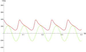
Fig 3: Replication of the plot presented by the Electric Druid. Red curve: modulated frequency for a 220Hz input frequency. Green curve: the modulating waveform (arbitrary units). It’s so accurate that even the colors are replicated!

Plot of modulation options — Fig 4: Black curve: pitch shift when modulating the period as in the Junos. Black dashed curve: pitch shift when modulating the clock frequency. Orange mess: the modulating waveform (arbitrary scale) and the same shifted with the sample line delay. Parameters are very coarsely Juno’ish.

So that’s the secret of the Juno style choruses! In addition to the heavily bandlimited delay line itself, it’s actually modulated in such a way as to give an essentially perfectly constant pitch shift (in the frequency range that the bandlimiting passes), which is of course exactly what would happen if you had two (because of the stereo delay line) extra oscillators. The only deviation is at the turning points, but those are of course necessary since the clock rate can’t endlessly increase or decrease. The more usual frequency modulated BBD in contrast has the pitch meandering restlessly, instead of a constant detune.

I also did some more work in solving the delay equation with some approximations to make it tractable, but I won’t bore you except by saying that you can get a nice expression for the pitch shift by approximating that $d w^{\prime\prime}(t) \ll w^\prime(t)$ , where $w(t)$ is the modulation waveform, and Taylor expanding $w(t)$ inside the integral around the output time $t$ , after which you can solve for the delay with no further approximations as (when doing the Roland -style period modulation)

$d = (1 + k w(t)) d_0 \frac{1 - e^{-d_0 k w'(t)}}{d_0 k w'(t)},$

where $k$ is the modulation index and $d_0 = \frac{N}{f_0}$ the base delay when modulation is at zero, i.e. $f_s(t) = f_0/(1 + k w(t))$ . Inserting that result to the pitch shift formula also proves that the pitch shift in the triangular modulation, when far from the turning points, is actually precisely constant.